Don’t wait for statistical significance (and other A/B testing lessons learned)

A few months ago, I started conducting formal A/B tests at work. I approached these experiments in the same manner as science experiments at school: assign queries to a control and test group, apply a treatment, observe a difference, and ascribe the difference to the treatment (loosely using statistical significance to distinguish treatment from randomness).

During those first few months of experiments, I made release decisions without a full understanding of a few fundamental A/B testing concepts. For example, I didn't understand the relationship between baseline conversion rates, false positives/negatives, minimum effect size, and sample size; or why I shouldn't "wait for significance" before concluding an experiment; or why I shouldn't interpret "not statistically significant" as "no effect." Below, I've tried to distill some of the more useful lessons that I learned using as little math as possible.

The root of many problems: sampling and chance

For the majority of my experiments, I'm interested in determining how often one of two possible outcomes occur. Did we show something or not? Did a user click or not? By the end of each experiment, I want to know if a change that I made increased, decreased, or did not change an existing metric.1 Making this determination often entails drawing conclusions based on sampled data. Here are several examples of some problems that might occur due to sampling and chance.

1. Variance: even if we know the rate of a particular user behavior or metric, we aren't guaranteed that we will always observe this rate. For example, assume that users click on a message every other time that the message is shown. With respect to sampling user behavior, clicking one-half of the time is similar to flipping a fair coin. The examples below will heavily draw on this analogy, switching between coin flips and user clicks. On average, we expect to observe the same number of clicks (heads) and did-not-clicks (tails). But, flipping a fair coin does not always produce an equal number of heads and tails:
   flips, chance for heads: 0.5 | Flip Again
   And the fewer the number of samples that we take, the more drastic the difference compared to our expectations:
   10 flips, chance for heads: 0.5 | Flip Again
   Not always observing the same number of heads and tails from a fair coin (more generically, the control group) complicates attempts to distinguish fair coins from unfair ones (more generically, the test group). Compared to the fair coin flips above, is it obvious that the flips below come from an unfair coin?
   Chance for heads: | Flip Again
   When we draw samples from two groups and compare—such as counting heads from a fair and an unfair coin, or counting clicks before and after a feature change—we are drawing conclusions based on an incomplete picture. Any similarities or differences that we observe may be due to the change that we made, or just to chance. There are two well known errors in A/B testing that are related to chance: false positives and false negatives.
2. False positive: we believe that a difference exists between two groups (that our change "really" has made a difference), when in fact it does not. We know that ten flips of a fair coin tend to result in a mix of heads and tails. If we see a run that is "very different" from this expectation—in the most extreme case, for example, a run with all heads or all tails—we might question whether our coin is actually fair. Observing a run of all heads or tails from a fair coin and concluding that it is not fair is an example of a false positive, and a run of all heads or all tails can happen more frequently than we might intuitively expect:
   10 flips, chance for heads: 0.5 | Start Trial
3. False negative: we believe that no difference exists between two groups (that our change did not make a difference), when in fact one does. If we have a fair and an unfair coin, and we observe runs that are "not different enough"—for example, both runs have the same number of heads and tails—we might believe that the coins have the same odds. Observing the same number of heads and tails between two coins with different odds and concluding that they have identical odds is an example of a false negative:
   Chance for heads:
   Chance for heads:
   10 flips | Start Trial

Sampling and chance can lead to misleading conclusions. It is impossible to rule out false positives and false negatives from A/B experiments whenever sampling is involved, and we will always have some uncertainty about the truthfulness of our experimental results. But, we can place limits on these uncertainties by judiciously choosing our sample size before conducting an experiment and then analyzing the experiment only after collecting enough samples.

The intricate relationship between sample size, false positives, false negatives, and other experimental parameters

False positives and false negatives are not topics that I thought much about prior to trying to learn more about A/B testing, and the examples above may still not sufficiently motivate why they're so important. The nutshell summary is that an intricate relationship exists between (1) an experiment's sample size, (2) the control group's underlying "conversion rate" (rate of heads, rate of clicks), the experimenter's willingness to observe (3) false negatives and (4) false positives, and (5) the minimum effect size claim that can be made relative to the control group's conversion rate at the end of the experiment. It is not possible to hold any four experimental parameters constant and simultaneously modify the fifth.

The most common example in my experience of modifying an experimental parameter with undesired consequences is stopping an experiment before collecting enough samples. In practice, assuming that most experimenters use commonly accepted maximum probabilities for false positives (5%) and false negatives (20%), stopping an experiment early necessarily means accepting a larger minimum effect size when interpreting "not statistically significant" results. But, when I started reporting A/B results, I never noted the minimum effect size as part of my results analysis. Only several months into testing did I start to learn not to interpret "not statistically significant" as "no effect," as well as about the dependence of the interpretation of "not statistically significant" on the minimum effect size parameter (discussed in greater detail below). For the highly curious, I wrote a Python simulation that explores the relationship between these experimental parameters in greater detail and shows the inner-workings of sample size calculators. We are always trying to measure if a difference exists between two groups while constraining the risk that we observe a false result, and these two goals always require more samples to achieve greater certainty.

Determining how many samples to take

If time, money, and resources were no matter, analyzing experiments after collecting an infinite number of samples would be wonderful. The more samples that we collect, the less uncertainty that we have due to sampling and chance. To illustrate why, the simulation below flips a fair coin 10,000 times and updates the chart with the total number of heads for each run. We know from earlier explorations that we will not always see an equal number of heads and tails; the simulation provides a visual representation of just how much of a deviation we can expect from run to run.

Unlike the ten-coin-flip examples earlier, if we didn't know that the coin in this simulation was fair, we could make a decent guess that the odds are nearly fair based on the observed percentage of heads and tails. The percentage of heads remains within a narrow range from run to run because we're taking more samples in each run. In general, the more samples that we take, the closer that our sampled rate approaches the actual, underlying (and usually unknown, in a real experiment) rate.

In many experiments, collecting more samples is not always feasible and has other trade-offs: for example, it may take more time or money, or there may not be enough available users. For A/B tests involving categorical questions that resemble coin flips, we can actually calculate how many samples we need based only on our experimental parameters:

1. Underlying metric rate: this is the baseline metrics rate (of heads, clicks) in the control group that we will measure differences against.
2. Minimum effect size: this is the smallest change in the underlying metric that we want to be able to measure. At the end of our experiment, a "not statistically significant" result will mean that the control and test group are different by no more than this minimum effect size, and we will not be able to make a more precise claim.
3. alpha, the false positive rate: setting alpha limits the possibility of observing a false positive. Specifically, alpha=0.05 states that if we rerun our experiment 100 times, we only want to observe a false positive 5 out of those 100 times. alpha=0.05 is a well accepted value for experimentation.
4. 1-beta, the false negative rate: setting beta allows us to limit the possibility of observing a false negative. If we repeat our experiment 100 times, setting 1-beta=0.8 states that if our feature really does make a difference, then we expect to observe that difference in 80 out of 100 runs. 1-beta=0.8 (that is, beta=0.2) is a well accepted value for experimentation.

Having chosen parameters for the underlying metrics rate, the minimum effect size, and the tolerance for false positives and false negatives, we can use an A/B test sample size calculator, like the one below, to evaluate how many samples we need to collect before ending and analyzing an experiment. (At work, we also like this sample size calculator.)

About statistical significance: deciding whether or not a difference exists

At the end of an experiment, we have to decide if our experimental change is responsible for any observed differences in metrics between the test and control. If we observe that a metric is "very different," we may be more willing to believe that our change was responsible. Alternatively, if we observe that a metric is "not different enough" between the two groups, we might conclude that our change didn't make a difference. In the earlier false positive and false negative examples, we arbitrarily defined what scenarios would qualify as "very different" and "not different enough" based on how many heads or tails we observed.

Rather than the phrase "very different," statistical nomenclature uses "statistically significant." And rather than "not different by enough," statistical nomenclature uses "not statistically significant." However, we don't need to invent arbitrary thresholds of difference for categorical questions that can only be answered one way or another. If we are only comparing how often a coin flip comes up heads or tails, or whether a user clicks or doesn't, well-known statistical tests such as Pearson's Chi-square test can quantitatively evaluate whether two groups are different beyond what we would expect from just sampling and chance.

Pearson's Chi-square test provides a quantitative score to answer questions of categorical difference, such as, "If users in group A clicked 5 times out of 100, and users in group B clicked 20 times out of 100, how likely is it that group A and group B are the same?" Pearson's Chi-square test returns a probability commonly referred to as "the p score" that answers this question. Pearson's Chi-square p is the same as alpha for calculating sample sizes. The lower the p score, the more likely that the control group and the test group are different (and thus, we might infer that our change created the difference).

"Just significant" p scores

In frequent practice, p scores lower than 0.05 are considered "statistically significant," and p scores greater than 0.05 are considered "not statistically significant." Hazards of all varieties (moral, logical, experimental) exist around the binary and arbitrary cut off, and I try to always consider the implications of false positives and false negatives when releasing experimental changes with p scores hovering around 0.05. There is nothing particularly special about 0.049 or 0.051, except that one sits on one side of an arbitrary boundary, and the other...on the other.

p scores and magnitude of change

For differences that are statistically significant, the p score states nothing about the magnitude of the change in coin flips or clicks. The magnitude of a change can be determined by comparing the difference in the underlying metric between the test and the control.

A tangent about "not statistically significant"

"Not statistically significant" may be one of the largest misnomers in A/B testing. Interpreting a "not statistically significant" result requires knowing the original experimental parameters. Specifically, a "not statistically significant" result only means that the effect of a change is not outside the range of the underlying metric rate plus/minus the minimum effect size. A "not statistically significant" result does not imply that the experimental change has no effect! "Statistically significant" and "not statistically significant" are both equally meaningful findings for an experiment. This is why "waiting for significance" should raise red flags.

Wrong minimum effect size

At the end of an experiment, it's possible that we'll observe an insignificant difference that leads us to question whether we chose the correct minimum effect size. For example, perhaps the experiment will say that clicks dropped 0.1%, but the difference is insignificant. It's possible that we simply didn't collect enough samples based on our underlying metric rate for this difference to pass the Chi-square test.

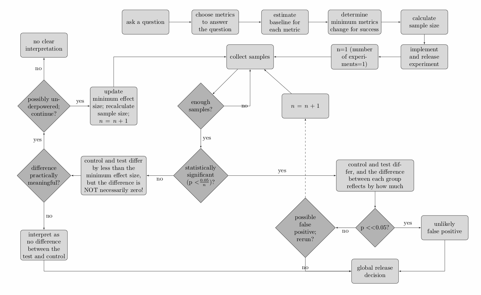
If, in fact, a 0.1% drop is meaningful and we chose the wrong minimum effect size, we should re-evaluate the number of samples that we need and whether we can continue running the experiment, or need to start fresh. In either case, we would likely need to lower the p score threshold to reflect the fact that we're drawing another experimental sample and increasing our chances of observing a false positive. If we do nothing at all and run an experiment 100 times with alpha=0.05, we expect 5 of these runs to result in a false positive. Our rerun is consuming one of these 100 runs. The simplest correction is to divide the starting threshold by the number of times we've rerun the experiment—for example, if we rerun it once, then we would use 0.05 / 2 = 0.025 as our new threshold for statistical significance.

Validating the claims of sample size calculators

We've outlined how to determine whether two groups are different with respect to yes/no questions, such as whether a user did or did not click. Along the way, we also reviewed problems that might arise due to sampling and noted that they can be mitigated by taking enough samples. But, we've taken for granted that sample size calculators "just work." How do we know that if we take the number of samples calculated, that we are guaranteed to observe our declared false positive/negative rate and be sensitive to our declared minimum effect size? Mathematical derivations do exist that explain how sample size calculators work, and they rely on well-known relationships between the mean and standard deviation of the binomial distribution. The simulations below take a less rigorous approach, running repeated trials to measure how often we observe false positives and false negatives under different sample sizes.

In the first set of simulations, we have two identical coins. Because we know the objective truth—the "control" coin and the "test" coin have odds equal to the baseline metric rate—any statistically significant differences that we observe represent a false positive. In the second set of simulations, we flip a "control" coin with odds equal to the baseline metric rate, and then on alternative tries a "test" coin that's either the baseline plus or minus the minimum effect size. Again, because we know the objective truth that the control and test coin are not identical, any run that ends with a not statistically significant difference is a false negative. On average, if we take the sample size calculator's prescribed number of samples, we should observe alpha fraction of false positives and beta fraction of false negatives.

The simulations above (made possible in part by Thomas Ferguson's Javascript implementation of the Chi-Squared distribution) show the last run with a false positive or false negative, as well as the overall rate of false positives and false negatives across all runs. Each run flips a coin in the test group and a coin in the control group the prescribed sample size calculator number of times, as well as half and double the calculator's prescribed sample size for comparison. The simulation compares the number of heads in the control and test using Pearson's Chi-square test for independence. In general, using the prescribed number of samples does constrain the number of false positives and false negatives as expected, and taking more samples is better than taking fewer. For the highly curious, I also wrote a more detailed Python simulation that explores the variance of false positives and false negatives within a series of runs.

Errors made and lessons learned

I made a lot of execution and analysis mistakes in the first few months of running A/B tests. I'm certain that I've made at least one in this blog post that I'm not currently aware of, and that there's a lot more to learn. I hope that others find this summary useful, and I welcome any suggestions for revision!

Next: Count Love: Aggregating protest data