
Dissertation distilled.
I wrote a monstrous document, circa 2015, about natural gas pipeline scarcities driving electricity prices higher and how to model the behavior of individual power generation firms that operate in tightly coupled natural gas and electricity markets. That document—my doctoral dissertation—is part linear programming, part economics, part policy analysis, and nearly two hundred pages long. Here, I’ve distilled that work into its most basic ideas for the curious.
The term “electricity market” tends to surprise people who have never heard it before. While not all electricity systems operate as markets, many, including most of the large systems in the United States, do. At any given instant, power generation firms want to sell electricity at different prices that largely depend on their costs, and consumers want to buy electricity for a wide array of end uses. The price that firms want to sell at and the price that consumers are willing to pay do not always match; firms that only want to sell electricity at high prices will tend to find few willing consumers, and consumers that only want to buy electricity at low prices will tend to find few willing suppliers. Electricity markets coordinate the behavior of generation firms and large consumers connected to the same transmission network by matching as many buyers and sellers as possible.
In practical terms, electricity markets coordinate the behavior of generation firms and consumers by determining the “marginal electricity prices” that buyers and sellers will trade with one another at throughout the day. These prices implicitly coordinate activity on the network because generation firms typically will not want to lose money by selling electricity when the marginal price falls below their cost, and consumers will not want to lose money by paying the marginal price for electricity when it exceeds the value that they would obtain from using that electricity.
Generation firms sell electricity at different prices because their costs to operate a power plant vary greatly depending on each plant’s technology. Some technologies, such as nuclear plants, have high, upfront investment costs and low fuel costs. Other technologies, such as natural gas, tend to have lower initial fixed costs but higher fuel costs. In addition to monetary differences, power plant technologies also vary widely with respect to the emissions that they create and their physical capabilities to start up, shut down, and operate somewhere in between these two states. All of these characteristics play an important role in determining how much electricity a firm can sell from each power plant. A lightbulb offers a succinct analogy to understand differences in power plant technologies. Consider two lightbulbs, one incandescent and one LED, both capable of producing the same amount of light. The incandescent lightbulb may initially cost less than its LED counterpart, but the incandescent lightbulb also costs more to operate per hour. Money aside, incandescent lightbulbs can also be easily dimmed over a large range of their total possible brightness, whereas LED bulbs have a smaller operating range and may require special dimming hardware. Diversity of power plant technologies allows a power system to balance operational reliability with cost, to adapt to changes in demand, and to react to unexpected supply interruptions.
Natural gas-fired power plants, one example of a fossil fuel power plant technology, operate by burning natural gas to generate heat, boil water, generate steam, and turn a turbine to generate electricity. Although the United States has abundant natural gas supplies, pipeline capacity to transport natural gas into some regions such as New England remains quite scarce because pipeline investment has historically required multi-decade agreements between industrial consumers, utilities, and pipeline operators. To date, power generation firms have benefited from the excess natural gas transport capacity that these other large-scale consumers created. However, over the last few years, as the power sector displaced all other sectors as the largest consumer of natural gas in the United States, investment in pipeline capacity slowed. This shift coupled the electricity market in regions with scarce pipeline capacity to the natural gas market. In particular, in New England, this coupling led to electricity reliability problems because 1) natural-gas fired power plants could not always acquire the fuel that they needed; and 2) due to economic and environmental factors, few alternative technologies remain that could substitute in for natural gas plants during pipeline scarcity events.
To explore the implications of such a tightly coupled natural gas and electricity market on potential pipeline investment and electricity reliability, I developed a computationally tractable, mathematical model of the decisions that a power generation firm must make in natural gas and electricity markets over a timescale ranging from a few hours to the next few years, taking into consideration uncertainty from future electricity demand, natural gas prices, pipeline availability, and unexpected power plant failures.
The model
Fortunately, I did not have to start from scratch. The field of electric power systems contains a few canonical mathematical models that describe optimal, welfare-maximizing decisions such as when power plants should turn on and off, how much electricity each plant should generate, and how much additional capacity should be built for each technology. Of course, these models are subject to strong assumptions, and they are necessarily always wrong in some manner. Yet, they are useful tools for exploration and discussion, so long as their results are interpreted with the correct skepticism and perspective.
Many electric power system models employ two central economic ideas. First, assuming a single central planner tasked with the goal of deciding everything—which power plants should turn on and off; how much each plant should generate; and which consumers will consume and how much—the central planner’s objective is to maximize the aggregate welfare of the electric power system. Welfare is defined as the revenue that firms earn less their cost, plus the utility that consumers gain less their cost. Second, under the assumption of perfect competition, a firm’s profit-maximizing decisions are identical to its decisions under a central planner’s welfare-maximization problem. With these economic ideas and assumptions, we can start our exploration of how to model the behavior of generation firms in a tightly coupled natural gas and electricity market.
I chose the canonical “unit commitment” model as the foundational building block for my dissertation because of its relatively fine temporal resolution. Broadly, the unit commitment problem answers the following question: given a power system’s power plants, their operating characteristics, costs, and the hourly electricity demand over a 24-hour period, when should each power plant turn on and off, and how much electricity should each plant generate in each hour to maximize welfare? Because the unit commitment problem contains a single, welfare-maximizing decision maker that knows everything about the power system, this type of unit commitment problem is often also called the “central planner’s unit commitment” problem.
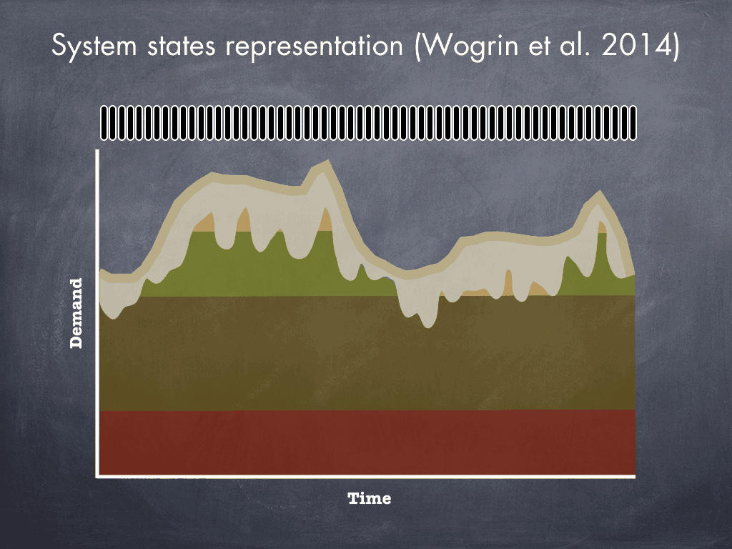
The central planner’s unit commitment problem can be mathematically expressed as a “mixed integer linear program.” Linear programs are special math problems that computers can adeptly solve; the autolayout of graphical user elements for iOS apps is just one example of a common linear programming application in everyday life. The “mixed integer” modifier for “mixed integer linear programs” indicates that some decisions are binary/integer in nature. For example, a power plant can be “off” or “on,” but not somewhere in between. Importantly, linear programs can guarantee under specific conditions that a solution is optimal with respect to a particular objective, and solutions to linear programs automatically yield useful economic information in the form of marginal prices. This is exactly how system and market operators in real electric power systems both calculate and justify their marginal electricity prices (which implicitly decide which firms can sell electricity on any given day). The cartoon diagram below shows a stylized version of a unit commitment’s outputs, given information about total electricity demand and power plant costs.

A stylized illustration of the outputs of a unit commitment model. The top line represents total electricity demand. The colored bands below represent each power plant’s output for each time interval t. From time t to time t+1, if a band disappears, that plant shuts down. A solution to a unit commitment problem represents a welfare-maximizing power plant schedule that indicates, for an entire power system, which and when power plants should turn on and off, as well as how much electricity each plant should generate given its physical operating constraints, costs, and the total electricity demanded for each time interval.
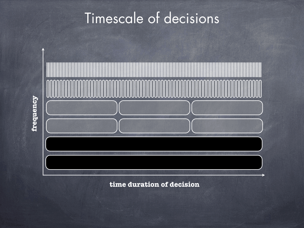
While most real-sized unit commitment models analyze one or two days at hourly intervals, generation firms must make a vast array of decisions that can span multiple years. Many of these decisions may require a firm to engage in a contractual agreement with another party before knowing what will actually happen in the future. To make well-informed decisions—for example, to balance the risk of paying too much to secure sufficient pipeline capacity ahead of time against the possibility of not needing that capacity in the future—generation firms must somehow take into consideration uncertainties such as future electricity demand, pipeline capacity availability, natural gas commodity price, and plant availability. The figure below shows the frequency and timescale of the primary decisions that I considered in the model developed for my dissertation.

Firms that own natural-gas-fired power plants must make a variety of long- and short-term decisions related to fuel, maintenance, and operation. Some decisions, such as how much electricity to offer into the market, must be made for every hour. Other decisions, such as whether to purchase long-term pipeline capacity or not, are only made once and will last for many years afterward.
A straightforward approach to model a firm’s multi-year and annual decisions would entail extending the hourly unit commitment model from twenty four to tens of thousands of hours, as shown in the figure below. New decision variables corresponding to the appropriate long-term decisions described above could be introduced spanning the appropriate number of hours. Unfortunately, this brute-force approach also requires computing a solution to the hourly unit commitment problem for tens of thousands of hours, which quickly turns into an intractable problem for any real-sized power system.
System operators typically run a unit commitment for the next twenty four hours. Extending the unit commitment problem to model decisions that can span multiple years would expand the number of short-term, hourly decisions tens of thousands of times.
To work around the computational intractability problems, I restructured my embellished-and-extended unit commitment formulation into a series of hierarchical optimization problems based on a dimensionality reduction approach first described in “A New Approach to Model Load Levels in Electric Power Systems With High Renewable Penetration” by Wogrin et al. in 2014. In that paper, the authors solve the unit commitment problem by first approximating it using system states. Rather than make one set of plant commitment and generation decisions per hour, they bin each hour into one of K-means clustered states, and then rewrite the unit commitment problem as a mixed linear integer program operating over only those states. The figures below illustrate how this state-based approximation works.
In a typical unit commitment, a solver must compute binary decisions for whether a plant should turn on or off and continuous decisions about each plant’s generation level for every hour (shown stylistically in black above).
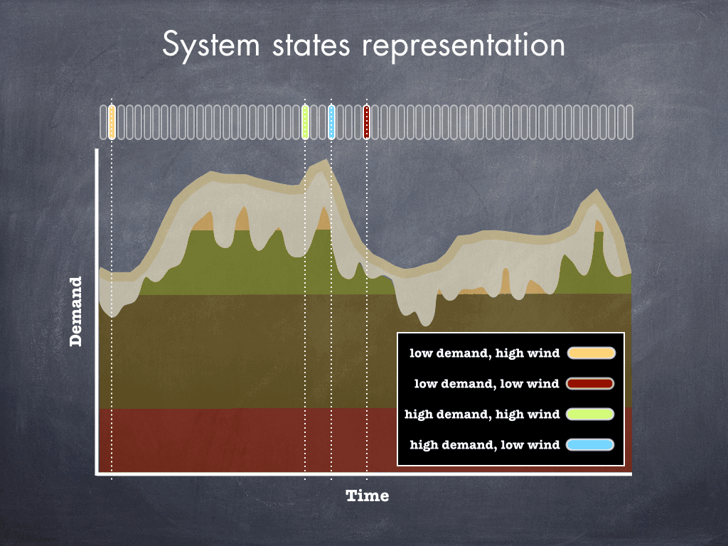
The system state approach reduces the number of decision variables, and consequently the computation time required, by approximating the hourly unit commitment problem and solving the approximation. After selecting a set of important power system attributes, such as the total electricity demand and wind generation level, a K-means algorithm picks K states that in aggregate represent the power system at different times. In the example above, K=4, and the K-means clustering creates four states in which wind generation is either high or low, and electricity demand is either high or low.

Once the K-means clustering algorithm picks its states, each hour of the unit commitment problem is categorized and binned into one of the K selected states. In this example, each hour of the power system is represented as either a low demand, high wind hour; a low demand, low wind hour; a high demand, high wind hour; or a high demand, low wind hour.

To recreate the time dynamics of the power system in the approximated unit commitment problem, for each month, the algorithm counts the number of hours spent in each state and the number of transitions between states. Then, the unit commitment problem is rewritten to consider the total time duration that the power system spends in each state and the frequency of transitions between states.
This state-based approximation, though not without its limitations, substantially reduces the amount of time required to solve a time-extended unit commitment problem. To analyze the multiyear, annual, and hourly behavior of generation firms, I constructed a hierarchical model that first solves for longer term decisions by approximating the shorter term problems using system states, and then reintroduced those longer term decisions as fixed parameters into the remaining shorter term problems. This approach allows longer term decisions to take short-term dynamics and uncertainties into consideration, while also allowing longer term decisions to influence a firm’s short-term choices. The figure below illustrates the final, hierarchical structure of the optimization model that I constructed to study the behavior of generation firms across multiple timescales.

A hierarchical representation of how to model decisions across multiple timescales for power generation firms, starting with a unit commitment. Inputs from the short-term model are approximated using system states as necessary to make medium- and long-term decisions, and those decisions are fixed and reintroduced as parameters into the shorter term, higher temporal resolution models.
Finally, to take uncertainties about electricity demand, natural gas commodity price, available pipeline capacity into consideration, I converted my embellished-and-extended unit commitment problem into a “deterministic-equivalent” mixed integer linear program. This modified the overall optimization program by forcing the solver to choose decisions that would maximize the weighted sum of welfare across all scenarios. A bit of jargon, but, pared down, instead of pretending to know what the future would look like at an hourly level for the next three years, the firm faced several possible future scenarios for electricity demand, natural gas commodity price, and pipeline availability.
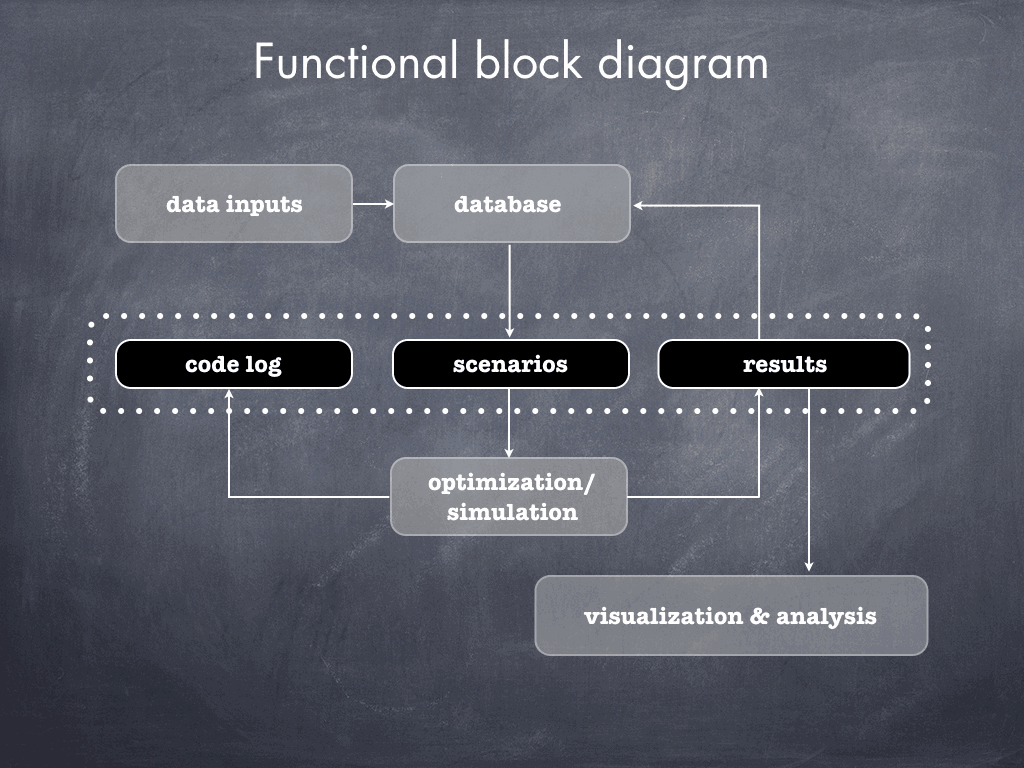
I wrote all of the actual, computable models for my dissertation in GAMS (General Algebraic Modeling System) and solved them with CPLEX, a commercial solver for linear and mixed integer linear programs. Inspired by the polling and prediction tools that I built for my NextBus Delay Tracker, I also built a research system, based on mySQL, Python, Git, and bash scripting, that automatically logged code changes, could reliably select and recreate scenarios, and would import and generate visualizations of my model’s outputs. The figure below shows a high level view of the different components involved. This research system saved me an incredible amount of time and allowed me to conduct, log, and review and reliably reproduce the results of hundreds of optimization runs (and I had a great time building it!).
This is the part of my dissertation that I had the most fun with, and probably the part that I am the most proud of. Just prior to having completed the mathematical formulation for my dissertation, I had developed a bus tracker to examine public buses as a break from my dissertation. It seemed fairly easy to take what I learned from that work and apply it to my research, and it turned out to be extremely fruitful—I was able to run optimizations easily without worrying about tracking uncertainty scenarios, regenerating inputs reliably between runs, and potentially losing track of what combination of model version and inputs produced which results.
Over the course of my dissertation, I ran over 400 different optimizations to explore how firms changed their behavior subject to different electricity demands, natural gas costs, and pipeline availabilities. I also explored how firms might react to different policies by holding all but one constraint constant, rerunning the optimizations, and then comparing how the objective function and decisions changed from run to run. While I did study New England as a case study for regions with tightly coupled natural gas and electricity markets, more generally, I built a set of tools to study the behavior of generation firms over multiple time scales with fine grain temporal resolution.
Intrigued? Read the entire dissertation or check out an example optimization model!